This will be a post about category theory and the relation between it and functors, monads and monoids in Haskell/Scala. This will be kind of a long post but i’ll cut the unnecessary details as much as possible. This first part is to talk more about theory and haskell relation between monads, functors and the category theory behind them.

Category Theory: Definitions

Components of a Category

Categories can be summed up as simple collections, that have the following components

• A collection of objects, obj ((C))
• A collection of morphisms, that are caled in other computer science literature as arrows, each of which can tie two objects, a source/target object, together. We can write it as:

For these functions we have that A is the domain and B is the codomain of f. The collection of arrows in a category C is denoted by Arr(C)

• For each object in the category, they have an identity arrow where the domain an codomain is the same object, thus:

• A notion of composition of these morphisms/arrows. For eg. if we have these 2 morphisms:

We can have a composed morphism of the previous two resulting in the following morphism:

These are only the mosaics to build categories, as these rules gives some kind of freedom of what type or other properties can the categories have. These are only very basic properties that any category should have to be considered one.

As we see these arrows, it may seem that they are always functions, but these needn’t to be the case. For example, any partial order ((P, \leq)) defines a category where the objects are the elements of P, and there is a morphism between any two objects A and B.

Category Laws

There are three laws that the categories need to follow.

Associative law

Based on the following arrows:

The composition of morphism needs to be Associative. Thus:

Morphisms are applies right to left in most of mathematical notications and conventions and in haskell. So if we have a composition like

g is applied first and then f.

Closed

Under these compositions

and

then we have a morphism h where

as seen by the composition property we can have this following representation of the category:

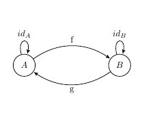
if now f and g are both morphisms we can compose them and get another morphism in the category so which is the morphism of f o g ? The only option is id((A)). Similarly g o f = id((B))

Identity

based on the identity rule we saw previously, if we have something like

Then we can sum up this law by:

A simple example

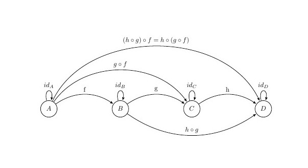
We can have the following category:

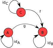
Where this is a category, with three objects A, B and C, three identity morphisms:

and morphisms

We can then compose f and g functions to build up a composition

We can see that we have even mosphisms for neutral elements or better called identity morphisms, for both A and B objects.

Commutative diagrams

Before moving foward with the category theory we can also represent the associative and identity laws by a directed graph diagram, where the law of composition is

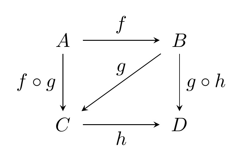
and the law of identity is for ex:

We can see in both of these diagrams that the path with the same source and destination is equal, thus they are commutative, this is only true on the case we mention and also that all directed paths in the diagram with the same start and endpoints lead to the same result by composition. Geometrically a diagram is commutative if every polygonal subdiagram is commutative.

Categories everywhere?

Now that we have seen the composition and laws that the categories should have we can mention some of the categories defined and existant even in Haskell. We can mention some examples like:

• Categories freely generated by directed graphs.
• Degenerate categories such as:
• • Sets – ie categories where all arrows are identities.
• • Monoids – ie categories with only one object.
• • Preorders: categories with at most one arrow between every two objects.
• 0, 1, .. , ω.
• Opposite categories C op: obtained by reversing the arrows of given categories C, while keeping the same objects.
• Set: the category of, sometimes small, sets and functions; composition is the usual function composition, and so is in the remaining examples. Note that type matter: the identity on the natural numbers is a different function from the inclusion of the natural numbers into the integers.
• Set∗: pointed sets, ie sets with a selected base-point, and functions preserving the base point.
• N: finite ordinals and functions.
• FinSet: finite sets and functions.
• Preord: preorders and monotone functions.
• Poset: partial orders and monotone functions
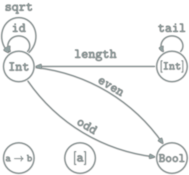
• Hask: Category for defining haskell types

These are some examples only to mention we’ll go deeper into some of them later but what are the differences of each of them? Well mentioned before the characteristics of the category and laws that it’ll have to comply are only the barebones of a category, we defined composition, arrows and objects at an abstract level but in reality each category will define what are it’s objects, arrows and how they can compose, these implementations vary depending on the category. We can see that even there is a category for the type declarations on Haskell, we’ll go into this later on..

for now lets go with a small exmaple, in this case Strings… for strings we have that the objects is represented by ob(Str) where the element could be represented by any string value, so if the object is the type only all the objects of this category will be only one: Str, so we can say this is only a singleton. Now the values that are for that type are any string value, so hom(Str) will be each string we can possibily build, that’s why we can say that ω will represent all the possible string values. Now our small category will need a composition (o) value which will be the concatenation in this case (++). So if we want to represent this category we can do like this following image, the w is actually

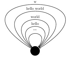
Now let’s try to see if the category laws can be verified:

For identity we had that:

now the id for Str will be

perfect the empty string is actually the identity, this will vary depending on the category, now lets prove it for any string z, lets see if the law can be verified:

allright, now lets try to demostrate if the associative law can be validated for any three strings.

for strings x,y and z we have that

So summing up this string example is kind of small but we can see that even with infinite paths, actually arrows, we can demostrate that the laws of category are respected. For a finite example we have that for a given category X

• ob((X)) = {A, B, C} these are the objects and represent the vertices of the diagram
• hom((X)) = {ε,α,β,γ,αβ,βγ,…} and each of these elements represent a path between the vertices.
• and finally the concatenation for ie. αβ∘γ=αβγ

Monoids

When the small example of Strings where shown, we said that they could be categories with a single value, we demonstrated that for all the strings that we can form, thus we can say that these are a spacial class of categories called Monoids, the axioms required of a monoid operation are exactly those required of morphism composition when restricted to the set of all morphisms whose source and target is a given object, that is that a monoid is essentially, the same thing as a category with a single object.

More precisely, given a monoid ((M, •)), one can construct a small category with only one object and whose morphisms are the elements of M. The composition of morphisms is given by the monoid operation •. These degenerated category, can be thought as a concept in which the categories are an extension of monoids, that can be generalised to small categories with more than one object.

some examples can be seen in this wikipedia link

With a more formal approach we can say that each monoid is represented by the triplet ((M,e,⊙)) where ob((M))={∙},hom((M))=M,∘=⊙

Examples of a monoid could be something like ((String, ‘Hello’, ++)) or ((String, ‘Something’, ++)), and in a more general way something that understands ((A, v, ⊙)), where A is the obj or class, v a value and ⊙ a way to compose with other monoids.

Monoids are very common. There are the monoids of numbers like N, Q, or R with addition and 0, or multiplication and 1. But also for any set X, the set of functions from X to X, written as

is a monoid under the operation of composition. More generally, for any object C in any category C, the set of arrows from C to C, written as Hom C (C, C), is a monoid under the composition operation of C.

Isomorphisms

In a category C, if we have an arrow of f : A → B, we can say that it’s called an isomorphism if there is an arrow g : B → A in C, that

Since the inverses are unique, we write (g = f^{−1}). We say that A is isomorphic to B, written A≌B, if there exists an isomorphism between them, where = is mostly ≌. The definition of isomorphism is our first example of an abstract, category theoretic definition of an important notion. It is abstract in the sense that it makes use only of the category theoretic notions, rather than some additional information about the objects and arrows.

Choices and other properties of categories

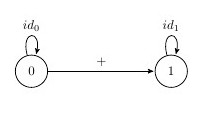
We can define that Integers can be saw as monoids, where the type is the object set of the category, meaning ob((Int)) is a singleton or either each of the numbers as a new category, for example, 0 could be a category with only it’s identity, and a category where 0 and 1 are objects and have the composition where you can compose both objects with a + function, these are two different categories, but you can also form a monoid based on Intgers where the value 0,1.. etc is actually not an object but instead the morphism, on integers that could be seen as monoids we can say that ((Integer, 0, +)) could be seen as a monoid too, so the same object can be seen in many different way as a category and also you can choose what are object, morphisms and composition, this applies only when you can prove that the categories laws are proveed and verified. Some examples of these besides Integers are Str and discrete((Σ*))

A category will also have properties based on their objects, morphisms and composition.

Initial and terminal symbols

An object is initial in a category C if for every object X in C there exists a unique arrow in C from it to X. Note that initial objects are unique up to isomorphism. The notation for ‘the’ initial object is 0, and 1 for ‘the’ final object, about this, an object is final, or terminal, in a category C if for every object X in C there exists a unique arrow in C from X to it, again there could be or not initial and final objects, then we can say that: A final in C iff A initial in (C^{op})

so final objects are unique up to isomorphism too. The initial object in a preorder is the bottom element, if it exists; the final object is the top.

Duality principle

First, let us look again at the formal definition of a category: There are two kinds of things, objects like ob((C)) = { A, B, C } and arrows hom((C)) = { f, g, h, …}, four operations dom(f), cod(f), id , g ◦ f, and these category properties satisfy the following seven axioms of the duality principle:

The operation (g ◦ f) is only defined where

so a suitable form of this should occur as a condition on each equation containing ◦, as in:

Now, given any sentence Σ in the elementary language of category theory, we can form the “dual statement” Σ ∗ by making the following replacements:

• (f ◦ g) for (g ◦ f)
• cod for dom
• dom for cod

It is easy to see that then Σ* will also be a well-formed sentence. Next, suppose we have shown a sentence Σ to entail one Δ, that is, Σ ⇒ Δ, without using any of the category axioms, then clearly Σ* ⇒ Δ* , since the substituted terms are treated as mere undefined constants, so we have for all the axioms showed for a category named CT that

We therefore have the following duality principle.

Functors… the category theory approach

Shamessly taken from https://en.wikibooks.org/wiki/Haskell/Category_theory

Well finally we can transform categories into another type of categories, for these exists the functors. We’ll see in this small section theorically what a functor does, later on we’ll see how functors work on Haskell, let’s see a functor ransforms a category A into a category B in this way bu a functor F:

The functor will do the following on the transformation:

• Maps any object A in C to F((A)), in D.
• Maps morphisms (f : C \rightarrow D) in A to F((f)): F((C)) (\rightarrow) F((D)) in B.

See this example:

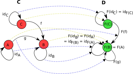
A functor between two categories, (C) and (D). Of note is that the objects A and B both get mapped to the same object in (D), and that therefore g becomes a morphism with the same source and target object, but isn’t necessarily an identity, and (id_A) and (id_B) become the same morphism. The arrows showing the mapping of objects are shown in a dotted, pale olive. The arrows showing the mapping of morphisms are shown in a dotted, pale blue.

For any category C, we can define a functor known as the identity functor on C, or (1_C : C \rightarrow C), that just maps objects to themselves and morphisms to themselves. We’ll use this later on monads.

Once again there are a few axioms that functors have to obey. Firstly, given an identity morphism (id_A) on an object A, F((id_A)) must be the identity morphism on F((A)):

also functors understand composition and must distribute over their morphisms:

One last thing to remember, there are some functors that will transform from one category A to another category A, these are called endofunctors.

Now for some more small demonstration of functors, given two categories A and B we can demosntrate that these have the following rules verified:

and

the functor F that transforms from one A to B will have a function called map that will make the following transformations:

Transform the composition operator after trnasforming it’s objects and arrows:

and also transform the identity:

Haskell time

We have seen some pretty long explanaition of introductory category theory, how does this has to do anything with Haskell code. In fact what I mentioned in the beginning was that there is a Hask category, let’s see what is it.

Hask category

Shamessly taken from wikibooks of haskell

Hask category treats Haskell types as objects and Haskell functions as morphisms and uses for composition ((\circ)) the function ((.)), a function (f :: A -> B) for types A and B is a morphism in Hask.

We can prove the composition between functions for eg that h = f.g, on the Hask there is also the identity ob an object defined by id, in Haskell

id :: (a -> a)
id x = x

The function id in Haskell is polymorphic — it can take many different types for its domain and range, or, in category-speak, can have many different source and target objects. But morphisms in category theory are by definition monomorphic — each morphism has one specific source object and one specific target object. A polymorphic Haskell function can be made monomorphic by specifying its type (instantiating with a monomorphic type), so it would be more precise if we said that the identity morphism from Hask on a type A is (id :: A -> A). With this in mind, the above law would be rewritten as:

(id :: B -> B) . f = f . (id :: A -> A) = f

If we want, we can also check the types of composition

(.) :: (b -> c) -> (a -> b) -> (a -> c)
(f . g) x = f (g x)

if we want to prove if the laws of categories are complied

-- left identity 
id . f = f 

= \x -> id (f x)
= \x -> f x
= f

-- right identity

f . id
= \x -> f (id x)
= \x -> f x
= f

-- associative law

(f . g) . h
= \x -> (f . g) (h x)
= \x -> f (g (h x))
= \x -> f ((g . h) x)
= \x -> (f . (g . h)) x
= f . (g . h)

Now types can define a lot about what is the behaviour of our functions in Haskell, some example could be the first function

Prelude> :t fst
fst :: (a, b) -> a

given a tuple of a type variable a and b as first and second member it returns the first element which is of type variable a. If you don’t exactly recall of know about type variables in haskell, you could look up in this section of learn you some haskell http://learnyouahaskell.com/types-and-typeclasses#typeclasses-101. Types can give you some good information about what the function expects and returns, what it’s important is that with type parameters we can generalize a function to handle different types, for eg. fst accepts a tuple if ([Char], Integer), for example:

Prelude> :t fst ("Hola", 1)
fst ("Hola", 1) :: [Char]

a is resolved to ([Char]) and b as Int in this case, so the type that will return fst is ([Char]), we’ll talk about this in the end of this post.

Another paper that you could read more about this is in Theorems for free

The Functor… typeclass in Haskell

typeclases

A typeclass is a kind of interface that defines a behavior, if a type is part of a typeclass, it’ll support and implement the behavior that describes the typeclass. This can be somewhat confusing for people coming from the object paradigm, so the typeclases are as Java interfaces, but implementing the behavior and not only defining your contract. Yeah, i know this is kind of an ugly comparison but if you come from an almost pure object paradigm it could be a little difficult to understand at first.

Prelude> :t (+)
(+) :: Num a => a -> a -> a

In this case + is a function that has a as a type variable and a type constraint that a can be of type Num or derivated from it, let’s see another example now:

Prelude> :t (<=)
(<=) :: Ord a => a -> a -> Bool

now this function is for comparing two different values of the same type that are of type Ord or derivated of this one. Ord is actually a typeclass and defines the prototypes for comparing two objects. Typeclasses are useful when defining new types for your own use as you can derive typeclasses to add not only the prototype of the typeclasses that you extend for your new type but also you can extend the typeclass by defining what it should do. In some cases you have to do this last thing. if you want to know more in depth and extense explanation about this see: http://learnyouahaskell.com/types-and-typeclasses#typeclasses-101.

Functors

let’s look a little what a functor is. Basically Functor is a typeclass to which you can apply the map operation. One would think that can be done in principle on lists, and this is what is usually seen in introductory functional programming material, but here we see that can also be used for other types, let’s see what the wiki says haskell:

More information on https://wiki.haskell.org/Functor

class Functor f where  
    fmap :: (a -> b) -> f a -> f b  

when we go to the part of the theory relate category, we see that the laws apply to this class:

fmap (f . g) = fmap f . fmap g  -- Composition law

fmap id = id                    -- Identity law

Fmap then takes a function that goes from a -> b, and a functor applied with one type, and returns a functor applied with another type. See the case for map

Prelude> :t map
map :: (a -> b) -> [a] -> [b]

Interestingly, seen as also takes a function of a -> b, and a list and returns another list, actually map is a particular case of fmap, so map is also a functor and map is a fmap defined for lists.

instance Functor [] where
    fmap = map  

so we can use directly fmap for operating with the functor on the list class!

Prelude> fmap (*2) [1, 3 ]
[2,6]
Prelude> fmap (*2) [1]
[2]
Prelude> fmap (*2) []
[]

It happens when we do a fmap on a list, empty? returns an empty list, this is logical, but makes a list of type ([a]) to type ([b]), where a and b of the same type.

Maybe and Either

let’s see the Maybe structure:

data Maybe a = Just a | Nothing

What does this mean? Maybe a represents something that can be (Just), or not (Nothing). That is, if we think as a container, Maybe is a box that can contain zero or item. And if you think like a computer, a function that returns a computation represents Maybe that may or may not yield a result, ie, a computation that can fail. What is the difference between the Maybe and eg Boolean, or list the ways we define before? The data type does not define values, but new types, this is known as constructors type, so in this case may be of a type x, so if we have a Maybe Int can result in a Nothing or Just one Int. For example if we take the most basic example, the reverse, if the inverse of x is 1 / x, if x == 0 then, its inverse would approaching infinity. so we have a case in which the computer can fail, because you can not compute to infinity, then see how we can represent an inverse function using Maybe.

inverse 0 = Nothing
inverse x = Just (1 / x)

if we want to have Maybe to extend the idea of the functor we need to implement fmap for this type:

instance Functor Maybe where
    fmap :: (a -> b) -> (Maybe a -> Maybe b)
    fmap f (Just a) = Just (f a)
    fmap f Nothing = Nothing

fmap (*2) (Just 1) == Just 2
fmap (+1) Nothing  == Nothing

now with either structre we have that:

data Either a b = Left a | Right b deriving (Eq, Ord, Read, Show)

Either as we see is a data type that can have values ​​of two types, and use one at a time. It behaves like a box with two compartments, but use one disables the other and vice versa. Then, as container is quite obvious: it is that allows you to store one of two values. And as computing, a function that returns Either depicts a computer that can be successful or not, and deliver a result or an error may occur. By convention, the Left is the error and right is the correct value. mnemonic: Right also means correct English.

A simple usage is with the inverse again:

inverse 0 = Left "Arithmetic Error: Division by zero"
inverse x = Right (1/x)

we can also extend Either for use with the Functor typeclass:

instance Functor (Either e) where
	fmap _ (Left a) = Left a
	fmap f (Right a) = Right (f a)

So Maybe a is used generally to handle the absence of the value a, fo eg. null in other languages. Either is used more in favour to handle errors.

so in this case, Functor is a type class used for types that can be mapped over.

generally a Functor accepts any two concrete types, how is this known in such a generic style? We saw that values like 1, “Hello” have associated types that are seen as labels that enable to know which type is a value. Types also have labels that tell about if they are concrete types or derivated form another constructions, these are called kinds. Type constructors take other types as parameters to eventually produce concrete types, this is something that is resolved by these labels that the type have, it’s kind. Lets see a small example

Prelude> :k [Char]
[Char] :: *

The * means that ([Char]) is a concrete type and no other replacement should take place when we have a type variable in a function declaration. for example if we see Either:

Prelude> :k Either
Either :: * -> * -> *

Either takes two concrete types and return a concrete type, type parameters can also be applied partially:

Prelude> :k Either Int
Either Int :: * -> *

This is what happens when we use an Either based on it’s kind a type parameter can take the value of a Type, given that the structure we’re using is of it’s same kind, producing a concrete type, we can use Either with any type. Now let’s try to see the Functor typeclass in a more theoric way:

The typeclass Functor has the followind kind prototype and definition

Prelude> :k Functor 
Functor :: (* -> *) -> GHC.Prim.Constraint


class Functor f where  
    fmap :: (a -> b) -> f a -> f b  

now if we Functor is:

then the tuple (F, fmap) is a Hask functor if for any x :: F a

so summing up we can say that haskell Functors are endofunctors that map: (F :: A \rightarrow A) where A = Hask category, and the tuple (F, fmap) is similar to say (Object, Morphism) theorically.

Natural Transformations

Given two functors F and G that transforms between two different categories:

we can construct a mapping that we will call natural transformation ((η)) that will map between the functors ans will associate any X object in category A to a morphism in category B, that is:

We have that for any morhpism that (f: X \rightarrow Y) called the naturallity condition, thus we have that:

this is called naturality square, represented by the following diagram:

Some examples

Let’s say we want to make a transformation from a type List to Maybe and backwards, we should have something like:

listToMaybe :: [a] -> Maybe a
listToMaybe [] = Nothing
listToMaybe (x:xs) = Just x

maybeToList :: Maybe a -> [a]
maybeToList Nothing = []
maybeToList Just x  = [x]

Another example could be a natural transformation between Either and Maybe

eitherToMaybe :: Either a b -> Maybe b
eitherToMaybe (Right x) = Just x
eitherToMaybe _ = Nothing

maybeToEither :: a -> Maybe b -> Either a b 
maybeToEither leftValue = maybe (Left leftValue) Right 

Composition of functors

We want now to compose two functions that have the folowing prototype:

the composition would be:

as the function f takes a parameter of type a the output of f, in terms of the type b is the input for the function g. But doing something like:

doesn’t quite work, because g is expecting a b not an (F b). So let’s start with the composition of:

Where x is any value of type parameter a that is an input for function f. now if we now that (f x :: Fb), then we have to find how to apply F b to the function g somehow. What do have to do?

Again let’s see what we have:

we can use fmap that we saw previously

and in a more generic way.

if we take that

now we have that F (F\,c) as result with using the fmap, we need to get to F c that’s what g is returning, we can’t do anything with this but fortunately we have the join function:

join :: m (m a) -> m a

with this we can express:

◎ is called the Klesli composition, denoted by the folowing symbol in haskell (<=<).

this composition must obey the following properties:

finally the klesli composition is defined in this way in haskell:

-- | Left-to-right Kleisli composition of monads.
(>=>)       :: (a -> m b) -> (b -> m c) -> (a -> m c)
f >=> g     = \x -> f x >>= g

-- | Right-to-left Kleisli composition of monads. @('>=>')@, with the arguments flipped
(<=<)       :: (b -> m c) -> (a -> m b) -> (a -> m c)
(<=<)       = flip (>=>)

see Control.Monad for more information.

Monads

Given all the definitions we have defined already the monads. Monads are formed by the triplet ((M,⊙,η)), where:

• M is an endofunctor
• ⊙ is a natural transformation where (⊙: M × M \rightarrow M), for eg. join function
• η is a natural transformation where η:I→M and I is the Identity functor

the rules that must obey this category are as alway associative and identity rules:

so a monad is an endofunctor M: C -> C and we have for every object in it’s category two morphisms:

• (unit_{X}^{M} : X \rightarrow M(X)) unit is actually the η ransformation
• (join_{x}^{M} : M((M((X)) )) \rightarrow M(X) ) join is actually our ⊙ transformation

let’s see now how is this translated in haskell:

class Functor m => Monad m where
  return :: a -> m a
  (>>=)  :: m a -> (a -> m b) -> m b

We have a type constraint for m where it has to be a Functor, this is only to ensure that we have mapping of morphisms and objects. We see that return is the polymorphic equivalence to (unit_x) for any X. But out bind function, denoted »=, is not similar to the join function we defined previously. However, we have the join function defined for Monads in haskell, as the following:

join :: Monad m => m (m a) -> m a
join x = x >>= id

and we can recover join from »= and vice-versa:

(>>=) :: Monad m => m a -> (a -> m b) -> m b
x >>= f = join (fmap f x)

so in terms of matematical approach, we need to define unit and join to have a monad, and in haskell we need to define the return and »= functions. Any time you see in haskell something that receives an x and returns a M((x)) naturally and a transformation from (M(M(x))) to M((x)), you’re probably using a monad.

There is a lot of well documented information further for seeing the monadic laws and examples on https://en.wikibooks.org/wiki/Haskell/Category_theory#Monads and https://en.wikibooks.org/wiki/Haskell/Understanding_monads

I’ll continue with some more theory about monads, and klesli categories in the next post, but trying to make some more code in scala this time.

Where to go from here?

I’de recommend to see Stephen Diehl post about Monads: The hard way, as it takes some of the theorically principles i showed in this post with some more details on haskell implementation of how you can see the relation between the category theory and haskell code.

I’ll try to take a more practical approach on my next post with Scala

Bibliography

• Awodey, Steve (2006). Category theory. Oxford University Press. p. 11. ISBN 9780198568612
• Vinberg, Ėrnest Borisovich (2003). A Course in Algebra. American Mathematical Society. p. 3. ISBN 9780821834138.
• Lipovaca, Miran (2011). Learn You a Haskell for Great Good!: A Beginner’s Guide. ISBN 978-1593272838.
• Turi, Daniele. Category Theory Lecture Notes
• https://en.wikibooks.org/wiki/Haskell/Category_theory
• http://yogsototh.github.io/Category-Theory-Presentation
• http://www.haskellforall.com/2012/09/the-functor-design-pattern.html

• 2024 1
• 2019 2
• 2013 1